Volatility does not rise everywhere for the same reason or at the same time. Equity uncertainty can jump during a growth shock, rates volatility during a policy repricing, currency volatility during a regime change, and oil volatility during a supply disruption. A cross-asset dashboard helps distinguish a broad risk episode from a local event. The challenge is that the underlying measures often use different assets, option markets, maturities, trading calendars, and calculation methods.
Putting raw volatility percentages on one chart can therefore create a false ranking. A level that is extreme for an equity index may be ordinary for crude oil, and a rates measure may not even share the same units. The solution is not to erase the raw data, but to organize comparison in layers: first preserve each series in its native definition, then use percentiles or standardized changes for a common overview. This guide explains a visual system for doing both.
Start with a definition matrix
Before plotting, create a table with the index name, underlying instrument, market, horizon, option type, unit, source, publication time, and holiday calendar. Two indexes may both be called “30-day implied volatility” while using different settlement rules, strike filters, or underlying futures. A realized-volatility series adds another distinction because it is backward-looking. The definition matrix prevents a convenient label from becoming an assumption of equivalence.
The FRED chart of selected Cboe volatility indexes provides a simple way to view several selected Cboe volatility index series in one place. That combined chart is useful for orientation, but the series still need individual metadata and historical context. A cross-asset visualization should link every shorthand label to a definition panel. Users must be able to tell whether they are comparing equity, gold, currency, and oil option-implied measures or a mixture of implied and realized estimates.
Raw levels versus normalized states
Raw levels preserve economic meaning within each market. They are essential when a user needs to know the actual index reading or price-implied volatility. They are weak for ranking across assets because baselines differ. A percentile transforms each series into its position within a chosen history. A z-score expresses distance from a mean in standard-deviation units, but it can be distorted by skewed distributions and crisis outliers. Both depend on the lookback window.
A strong dashboard uses two views. The first shows small multiples in raw units with independent but clearly labeled scales. The second shows a common heatmap of percentiles or robust standardized values. Keep the normalization method fixed and display the lookback, such as five years of daily closes. Provide raw values in tooltips and a table so the common scale does not conceal the magnitude that portfolio and option decisions may require.
Heatmaps for breadth and synchronization
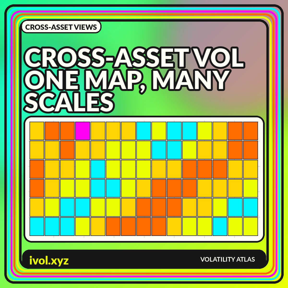
A heatmap with assets in rows and dates in columns reveals whether stress is broad or concentrated. A vertical stripe across many rows suggests synchronization; a single bright row suggests a local shock. Sort rows by asset class rather than by current value so the map remains stable over time. Use a perceptually ordered scale and include symbols or text for users who cannot rely on color alone.
Daily heatmaps can become dense over long histories. Aggregate to weeks for strategic views and keep a zoomed daily panel for current conditions. Missing observations should be visibly distinct from calm values; filling holidays with the prior close can create false persistence. If one market is closed while another reacts to news, the apparent lead-lag relationship may be a calendar artifact that resolves only when the closed market reopens.
Correlation is state-dependent
Cross-asset volatility series often become more correlated during broad shocks, but the relationship is not constant. Rates volatility can rise during either inflation concern or growth fear, with different implications for equities and currencies. Commodity volatility may be dominated by sector-specific supply events. A full-sample correlation matrix averages these episodes together and can hide the very state changes the dashboard is intended to reveal.
Use rolling correlations with several windows or compare matrices across predefined regimes. Report observation counts and avoid treating correlation as causation. Volatility indexes can share inputs indirectly through macro news, hedging demand, or global liquidity without one causing the other. A network diagram can highlight clusters, but a labeled matrix is easier to audit. Keep the asset ordering constant across dates so visual changes reflect data rather than layout.
Event alignment and lead-lag caution
To study a macro release or geopolitical event, align each series to a common event time and show changes rather than only levels. Publication times, option-market hours, and settlement conventions matter. A daily close in one region may occur before the event while another market's close occurs after it. Without timestamp alignment, a chart can incorrectly suggest that one asset anticipated another.
Intraday analysis requires even more care because liquidity varies through the global day. Use synchronized timestamps in UTC and note market-open status. Test lead-lag relationships across multiple events rather than selecting one dramatic example. A persistent visual ordering can still arise from reporting lags or stale indexes. The dashboard should communicate timing uncertainty instead of drawing arrows that imply a transmission mechanism the data cannot establish.
Changes, ratios, and volatility spreads
Level differences are not the only useful comparison. Daily or weekly changes show where repricing is most intense. Ratios can express relative uncertainty, such as one asset's implied volatility divided by another's, but a ratio becomes unstable when the denominator is low and can be difficult to interpret across structural breaks. A difference in normalized percentiles is often more robust for a broad monitoring screen.
Volatility spreads should be tied to a clear hypothesis. A widening equity-versus-bond volatility gap may reflect market-specific news, differing horizons, or methodology rather than a universal risk preference. Plot the two source series beside the spread and mark changes in index construction. Never present a spread without the components; otherwise users cannot tell whether it moved because the numerator rose, the denominator fell, or both changed.
From market map to portfolio context
A cross-asset volatility map is not automatically a portfolio-risk map. Portfolio impact depends on exposure, direction, convexity, correlation, liquidity, and hedges. A high percentile in an asset with no exposure may matter less than a moderate rise in a concentrated position. Add a separate exposure layer rather than recoloring the market data to imply portfolio importance without showing the weights.
For an allocation dashboard, combine each asset's volatility state with portfolio contribution to risk. Keep the market measure and portfolio measure in adjacent columns so users can see the distinction. Scenario panels can show how synchronized increases would affect estimated risk, but label assumptions and avoid presenting model output as a guaranteed loss. Stress tests should include correlation changes and liquidity constraints, not only a uniform volatility multiplier.
A practical cross-asset dashboard layout
Use a top row of current percentile cards, a central historical heatmap, and small-multiple raw charts below. Add a rolling correlation matrix and an event timeline as secondary views. Each card should show the raw value, percentile, date, delay status, and underlying definition. A user should be able to move from the common overview to the native series without losing context.
Keep the visual hierarchy disciplined. Bright colors should be reserved for unusual states, not every data point. Use the same date cursor across all panels and allow a selected event to create before-and-after snapshots. When data are illustrative, state that clearly in the chart itself. When data are live or licensed, show source and timestamp. Cross-asset breadth is valuable only when the dashboard makes differences as visible as similarities.
Conclusion
Cross-asset volatility visualizations can distinguish global stress from market-specific repricing, but raw percentages are rarely comparable without context. Definitions, horizons, units, calendars, and publication times must be aligned before a common heatmap or ranking is meaningful.
Preserve native series in small multiples, then add percentiles or robust standardized views for breadth. Show missing data, synchronize timestamps, and separate market state from portfolio exposure. The result is not one universal fear gauge; it is a layered map of how uncertainty is priced across different markets.