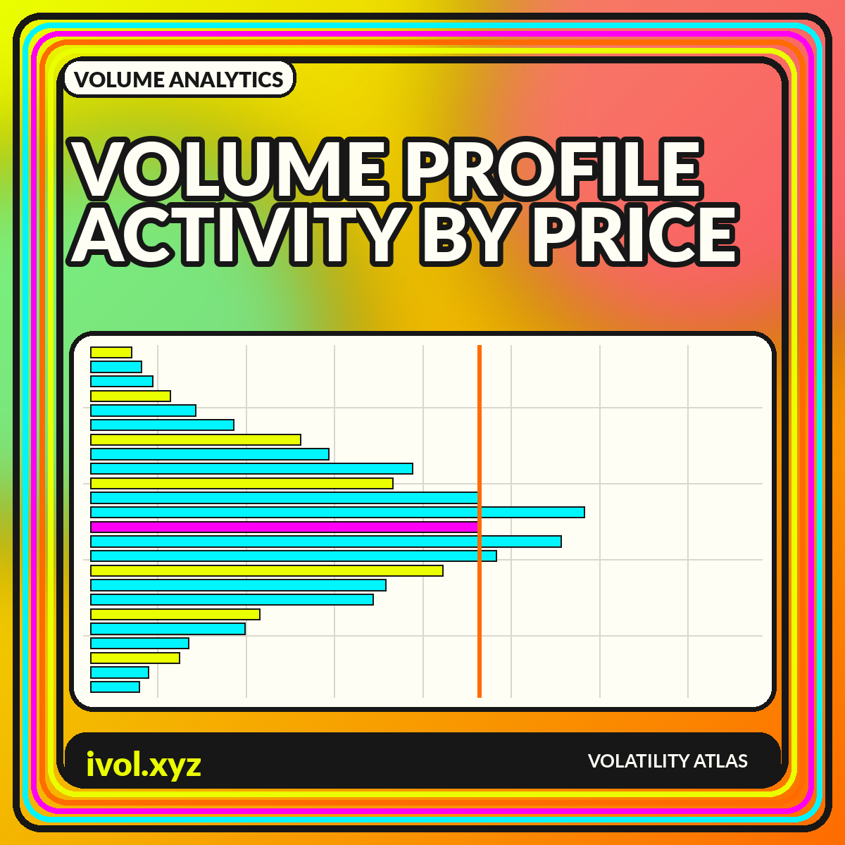
A conventional volume histogram tells you how much traded during each time bar. A volume profile reorganizes the same basic idea around price: it accumulates activity at price levels and draws a horizontal distribution next to the chart. The result can reveal where the market spent substantial effort, where it moved quickly, and how the chosen session or lookback distributed volume. The shape is descriptive. It does not convert historical activity into permanent support, resistance, or fair value.
Volume profiles are highly sensitive to their settings. Change the anchor date, session template, row size, contract treatment, or data coverage and the visible nodes can change. A responsible chart therefore exposes its construction rather than presenting the profile as an objective fingerprint. This guide explains the main labels, the role of anchoring, the difference between time and price distributions, and a workflow for using profiles as context instead of as standalone trade commands.
How a volume profile is constructed
The chart begins with trades that occurred inside a selected time range. Each trade's volume is assigned to a price row or bin. The total for each bin becomes the length of a horizontal bar. Because traded prices rarely align perfectly with a simple grid, platforms may allocate volume using tick-level records or approximate distribution rules based on lower-resolution bars. The method matters most when the input bars are wide or when the market moved rapidly through several price levels.
The Charles Schwab guide to the volume profile indicator introduces volume profile as a way to view trading activity at price levels rather than only through time. For reproducible analysis, record the instrument, venue coverage, time zone, session start and end, row-size rule, and whether the platform used actual trades or a bar-based estimate. Two profiles that look different may both be internally correct if they were built from different sessions or aggregation methods.
Point of control and value area
The point of control, often abbreviated POC, is the profile row with the greatest accumulated volume. The value area is a platform-defined price range intended to contain a chosen share of the profile's volume, commonly centered around high-activity rows. Value-area high and value-area low mark its boundaries. These labels summarize a distribution, but they do not imply that price is mathematically compelled to return or remain inside the range.
Always state the percentage and algorithm used to compute the value area. Some methods expand outward from the POC one row at a time; others use different selection logic. Ties and irregular profiles can create small differences between vendors. A chart should show the POC as a labeled line and the value area as a lightly shaded region, while keeping the full profile visible. Hiding the tails makes the central region appear more decisive than it really is.
High-volume and low-volume nodes
High-volume nodes are bulges in the distribution where the market recorded relatively heavy activity. Low-volume nodes are thinner areas where less trading occurred. Analysts often describe high-volume regions as areas of acceptance and low-volume regions as areas of rejection or rapid travel. Those interpretations can be useful narratives, but they are retrospective. The profile records what happened inside the selected sample; it does not guarantee the same behavior when price revisits the level under new information and liquidity conditions.
Node detection depends on smoothing and bin width. A very fine profile can show dozens of small peaks that are visually impressive but unstable. A very coarse profile can merge distinct auction regions into one broad block. Use sensitivity testing: display the result under at least two reasonable row sizes and focus on features that persist. When a key node disappears after a minor settings change, it should not be treated as a robust level.
Fixed-range, session, and visible-range profiles
A fixed-range profile is anchored to dates or bars chosen by the analyst. A session profile resets for each defined session. A visible-range profile recalculates whenever the user zooms or pans. These modes answer different questions. Fixed range can study a specific trend or event, session profiles compare daily distributions, and visible range provides quick exploration. The last mode is convenient but especially vulnerable to unintentional cherry-picking because the indicator changes with the screen.
For published research, fixed anchors are easiest to audit. Explain why the range begins and ends where it does—for example, an earnings gap, a contract roll, or a complete calendar quarter. When comparing sessions, use identical hours and account for early closes and daylight-saving changes. For markets with nearly continuous trading, decide whether to separate a primary cash session from the overnight session, since their profiles can have different liquidity and participant mixes.
Volume profile is not market profile
Volume profile and market profile can look similar because both produce horizontal distributions. A traditional market profile or time-price-opportunity chart organizes the amount of time or number of time brackets spent at each price. Volume profile organizes traded volume. A price can host many time brackets with limited volume, or substantial volume in a short burst. The measures may align, but they are not interchangeable and should not share a generic label.
A useful comparison places the two distributions side by side using the same price bins and time range. Differences reveal whether the market lingered quietly or transacted heavily. Add a conventional time-based volume panel to preserve the chronology that both profiles compress. A horizontal profile removes sequence: two sessions can create nearly identical distributions even though one moved upward first and the other moved downward first.
Composite profiles and evolving distributions
Combining several sessions can reveal a broader distribution, but the composite may hide meaningful regime changes. A month that includes both a low-volatility range and a later breakout can produce a profile whose central node belongs mostly to the earlier environment. Track the profile as it evolves or divide the sample into subperiods. Animated or small-multiple profiles can show whether activity is migrating upward, downward, or splitting into multiple accepted regions.
Developing POC and value-area lines can be plotted through time, but they are path-dependent. Today's developing POC can move after later trades accumulate, so historical lines should not be mistaken for values known with final certainty at every prior moment. In backtests, use only information available at the time and specify whether the profile resets. Recalculating a fixed full-sample profile and applying it backward creates look-ahead bias.
Data quality and fragmented markets
A profile is only as complete as its trade feed. U.S. equities can trade across many venues and off-exchange facilities. Digital assets trade on separate exchanges with varying quality and reporting conventions. Foreign exchange spot volume may be broker-specific or represented by tick activity rather than centralized transactions. Futures profiles must handle contract rolls. A chart that looks precise can still represent only one slice of the market.
Display venue coverage and distinguish consolidated from single-venue data. Remove or flag obvious bad ticks, but document the cleaning rule. For continuous futures, decide whether to profile each contract separately, combine contracts during the roll, or use a back-adjusted price series with original contract volume. Back-adjusted prices can shift historical levels, so plotting an old profile against adjusted prices may misalign the very levels the chart is meant to study.
A practical profile-reading workflow
Begin with price structure and choose an anchor that corresponds to the analytical question. Confirm the session and data source, then select a row size that produces a readable distribution without manufacturing detail. Mark the POC, value-area boundaries, and the most persistent high- and low-volume nodes. Compare the profile with range, trend, realized volatility, and time-based volume. The profile should add a price-distribution view, not replace the chronology of the market.
Before acting on a level, ask what new information has entered since the profile was formed and whether liquidity conditions are comparable. Treat a revisit as an observation point rather than a predetermined outcome. In a dashboard, make the anchor editable and show the resulting settings in the exported image. That simple design choice lets readers reproduce the view and prevents a visually compelling distribution from becoming an unexplained artifact.
Conclusion
Volume profile charts reveal where activity accumulated by price within a defined sample. The POC, value area, and high- or low-volume nodes are concise descriptions of that distribution, not permanent laws of market behavior. Their reliability depends on data coverage, row construction, session rules, and the analyst's anchor.
Use profiles alongside price path, time-based volume, volatility, and liquidity context. Publish the settings, test sensitivity to bin size, and avoid using a visible-range profile as hidden hindsight. When its construction is transparent, volume profile is a powerful map of historical participation—and a disciplined starting point for better questions about current structure.