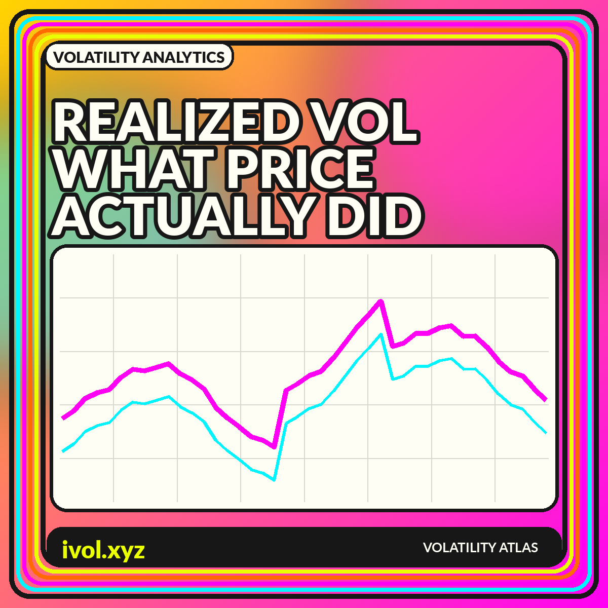
Realized volatility is built from prices that actually occurred. In its simplest form, calculate returns, measure their dispersion over a window, and annualize the result. The phrase sounds objective, but there is no single realized-volatility series. A 10-day close-to-close estimate, a 30-day range-based estimate, and a one-day measure from five-minute returns can all be correct while showing different levels and turning points. Every chart embeds choices about time, sampling, cleaning, and market hours.
Those choices determine what the visualization can support. A fast estimator can highlight current stress but will be noisy. A long rolling window will look stable but react slowly and contain overlapping observations. Intraday measures can capture more information yet become sensitive to microstructure noise and missing data. This guide explains the construction, comparisons, and design patterns that make realized-volatility charts interpretable rather than deceptively precise.
From prices to a basic volatility estimate
Most close-to-close estimates begin with logarithmic or simple returns. The standard deviation of those returns over a chosen window is then multiplied by the square root of an annualization factor, often based on trading days for daily data. The result is an annualized percentage. This scaling assumes a relationship between variance and time that is useful for comparison but imperfect when returns are autocorrelated, volatility changes within the window, or trading is discontinuous.
The NBER overview of realized return volatility discusses realized volatility as a way to use higher-frequency observations to measure return variation more directly. The basic principle is that squared intraday returns can be aggregated to estimate daily variation, subject to data and sampling limits. Whether using daily or intraday inputs, publish the return definition, sample frequency, lookback, and annualization convention. Without them, two lines labeled “realized volatility” cannot be meaningfully compared.
Rolling windows and the overlap problem
A rolling 20-day series shares 19 observations with the prior day's estimate. That overlap makes the line smooth and persistent even if the underlying returns are independent. It also means adjacent points are not separate experiments. A spike remains in the window until it ages out, sometimes creating a sudden drop exactly one lookback later. The chart can therefore show mechanical cliffs that reflect window construction as much as a current change in conditions.
Display multiple windows or an exponentially weighted estimate to show sensitivity, but avoid filling the page with nearly identical lines. A useful set might include a fast 10-day, medium 30-day, and slow 90-day measure. Label the lookbacks directly at the line ends. For statistical testing, account for overlapping data rather than treating every daily observation as independent. For communication, annotate when a major return enters and leaves the shortest window.
Close-to-close and range-based estimators
Close-to-close volatility ignores the path inside each session. Range-based estimators use highs and lows, and some incorporate opens and closes, to capture more of the day's information. They can be more statistically efficient under their assumptions, but they depend on reliable extremes and treatment of overnight gaps. A market with a short cash session and significant overnight news needs a different interpretation from a continuously traded market.
Instead of declaring one estimator best, match it to the question. Close-to-close is transparent and easy to reproduce. A high-low measure can describe intraday range more sensitively. An open-high-low-close estimator can use more fields but may assume a process that does not fit every asset. Plot a ratio or difference between estimators to find periods when overnight gaps or intraday swings dominate, and document how bad highs or lows are filtered.
Intraday sampling and microstructure noise
Using more frequent returns appears to offer more information, but sampling too finely can amplify bid-ask bounce, discrete pricing, asynchronous trading, and data errors. One-second returns may be dominated by market microstructure rather than the underlying price process. A coarser interval such as five or ten minutes can reduce noise, though the appropriate choice varies with liquidity and market structure. Sparse assets may require much wider intervals.
A volatility signature plot compares the estimate across sampling frequencies. If the value rises sharply as the interval becomes very fine, microstructure effects may be material. Keep session boundaries consistent and decide how to handle periods with no trades. For cross-asset comparisons, do not use the same frequency mechanically: a liquid index future and a thin individual token can have radically different trade intensity and quote behavior.
Annualization and the meaning of the percentage
Annualization makes estimates from different horizons easier to compare, but it can also create a false sense of forecast precision. A realized value of 25% over the past month does not mean the asset will move exactly 25% over the next year. It means the observed variance, scaled under a convention, corresponds to that annualized rate. A short burst of stress can generate a very high annualized number even if the episode lasts only a day.
State whether the factor assumes 252 trading days, 365 calendar days, or another basis. Around-the-clock markets often use calendar scaling, while exchange-traded assets may use trading days. If overnight returns are included, the trading-day convention still spans calendar time between closes. For a nontechnical audience, pair the annualized line with a realized range or cumulative-return panel so the percentage is connected to an observable price path.
Realized volatility versus implied volatility
Realized volatility looks backward over a chosen sample, while implied volatility is derived from current option prices for a forward horizon. Comparing them can be informative only when horizons and definitions are aligned. A 30-day implied measure should not be compared casually with a 10-day historical estimate or with realized volatility that includes an event outside the option window. The timing of observation also matters because implied volatility can change intraday while a daily realized estimate is fixed at the close.
A fair comparison can plot today's constant-maturity implied volatility against the subsequently realized volatility over that same future period. That creates a forecasting evaluation but introduces overlapping forward windows and requires careful timestamp alignment. A simpler live dashboard can show current IV beside trailing realized measures while clearly labeling one forward-looking and the others backward-looking. Avoid calling the difference a guaranteed premium; execution costs, jumps, skew, and path-dependent strategies matter.
Regime charts and volatility-of-volatility
Realized volatility tends to cluster: calm periods are followed by calm periods and turbulent periods by turbulent periods more often than a constant-volatility model would suggest. Regime bands or percentile zones can help summarize this persistence. Use rolling quantiles or a documented statistical model, and distinguish descriptive categories from predictions. A threshold estimated with future data should not be applied retrospectively as though it were known in real time.
Volatility itself can vary sharply, so a second-order measure such as volatility-of-volatility may help identify unstable regimes. Keep the hierarchy understandable: plot the primary realized-volatility series, then a smaller panel for its rate of change or variability. Too many derivatives of the same input can create an illusion of independent confirmation. The chart should reveal how the estimate behaves, not multiply one source of information into several apparent signals.
A clear realized-volatility dashboard
Use price or cumulative return at the top, realized volatility below, and a distribution or percentile panel at the bottom. Add controls for window, estimator, and session, but display the selected settings in the exported image. Highlight missing data and avoid drawing a continuous line through long gaps. If several assets appear together, use normalized percentiles for overview and provide raw annualized values in a table.
Charts should answer one of three questions: what happened, how unusual was it, or how did an estimate compare with another measure. A time series answers the first, a percentile or historical distribution answers the second, and aligned implied-versus-realized views answer the third. Keep those tasks separate. A single multiaxis panel with price, volume, two volatilities, and a regime score may look efficient but makes causality and scale impossible to judge.
Conclusion
Realized volatility is an estimate of observed price variation, not a unique fact detached from methodology. Window length, sampling frequency, session definition, estimator, cleaning, and annualization all shape the line. Short windows react quickly and noisily; long windows provide stability at the cost of lag.
Build charts that expose those choices. Compare like horizons, show sensitivity to reasonable settings, and pair annualized percentages with the price path that generated them. With clear metadata and disciplined panel design, realized volatility becomes a useful account of market behavior rather than an unexplained number that changes with the software default.