Implied volatility, usually shortened to IV, is the volatility level embedded in option prices. It is not a forecast that an asset will rise, fall, or finish at a particular number. It is better understood as a market-implied scale for uncertainty: the option market is assigning more or less price to the possibility of movement over a defined horizon. That distinction matters because a high IV reading can coexist with a bullish chart, a bearish chart, or a market that ultimately goes nowhere.
A useful IV visualization therefore begins with three questions: which underlying asset, which expiration, and which strike or summary measure? A single percentage without that context can conceal more than it reveals. The goal of this guide is to turn IV from an isolated quote into a visual framework. We will compare levels through time, study the shape across strikes, connect IV to expected range, and identify the charting errors that most often produce false confidence.
What implied volatility actually represents
An option price contains several moving parts: the underlying price, strike, time remaining, interest rates, expected distributions, and supply-demand pressure. In a pricing model, volatility is the input that reconciles those observable terms with the market price of the option. Solving backward for that input produces implied volatility. The result is quoted as an annualized percentage, but it belongs to a specific option and moment. It is not a universal property of the asset, and it can change even when the underlying price barely moves.
The most important interpretation is relative rather than absolute. An IV of 30% may be elevated for a slow-moving large-cap stock yet ordinary for a smaller growth company or a cryptocurrency. Context comes from the asset's own history, neighboring expirations, nearby strikes, and comparable instruments. Options Industry Council overview of options pricing explains how volatility is one of the factors reflected in option premiums. A chart should preserve that relationship by showing IV alongside time to expiration and price context, instead of presenting the number as a free-floating signal.
Why IV says range, not direction
Volatility measures the magnitude of potential movement, not the sign of that movement. A market can price a wide future range because participants see meaningful upside and downside paths. This is why the phrase “fear gauge” can be misleading when applied broadly: higher IV often accompanies stress, but it can also rise before earnings, court decisions, product announcements, elections, or any event that expands the set of plausible outcomes. Directional expectations require other evidence, such as skew, positioning, price trend, or a specific option structure.
On a dashboard, separate the range dimension from the directional dimension. One panel can show an at-the-money IV series; another can show the underlying return; a third can show put-versus-call skew. When all three are overlaid on one axis, users may mistake a rising IV line for a bearish forecast. Small multiples are clearer. They let a reader see that uncertainty can increase while price rises, decrease during a selloff, or remain high after an event if uncertainty has not actually resolved.
From annualized IV to an expected-move estimate
A common approximation converts annualized IV into a one-standard-deviation move for a shorter horizon. Multiply the asset price by IV and by the square root of time expressed as a fraction of a year. For a 20-day horizon, the time factor is the square root of roughly 20 divided by 365. The output is a price-distance estimate, not a hard boundary. It assumes a simplified distribution and does not account for every market feature, but it helps translate a percentage into a chart band users can intuitively inspect.
Expected-move bands should be labeled as estimates and tied to the IV input used. A 30-day at-the-money reading creates a different band from a 7-day event-heavy expiration. Use a centerline for spot or forward price, shaded upper and lower bands, and a caption stating the horizon and calculation convention. Avoid implying that the market assigns a fixed probability to never crossing the band; paths can move beyond it and return, and real return distributions can have asymmetry and fat tails.
Reading IV rank, percentile, and z-scores
IV rank places today's reading between the minimum and maximum observed over a chosen lookback. IV percentile reports the share of observations below today's level. They answer different questions and react differently to outliers. A single extreme spike can compress rank readings for months, while percentile is less sensitive to the magnitude of that spike. Neither statistic is meaningful without the lookback window, sampling frequency, and exact IV series used. A one-year percentile based on daily closing values is not interchangeable with a five-year intraday measure.
For visual comparison, show the raw IV line first and the normalized statistic below it. Add visible markers for major events rather than forcing users to infer why the series changed. A z-score can be useful when the distribution is reasonably stable, but volatility itself often changes regime, so a normality-based score should be treated as a descriptive transform rather than a probability statement. The chart title should state whether the series is at-the-money, constant-maturity, model-derived, or vendor-specific.
Term structure: comparing expirations
The IV term structure compares volatility across expiration dates. An upward-sloping curve means longer-dated options carry higher IV than near-term options; an inverted curve means the near term is priced more intensely. Event risk often creates a local hump at the expiration that contains the event. Broad market stress can invert much of the curve because immediate uncertainty dominates. The shape is more informative than a single point because it reveals where the market concentrates uncertainty in calendar time.
A clean term-structure chart uses days to expiration on the horizontal axis and comparable IV points on the vertical axis. Plot current, prior-day, and prior-month curves with restrained labeling. Do not connect expirations from different settlement conventions or underlyings without disclosure. For recurring analysis, constant-maturity interpolation can improve comparability, but the method should be documented. The reader needs to know whether a 30-day point is a listed option or an interpolation between surrounding expirations.
Skew and the volatility smile
Within one expiration, IV can vary across strikes. Equity index options often show higher IV for lower strikes, producing a downside skew. Other markets may display a smile or a more complex shape. This does not mean the option market publishes a literal probability distribution without assumptions; it means different portions of the payoff space trade at different implied volatilities. Supply, hedging demand, jump risk, liquidity, and model limitations all contribute to the observed curve.
Visualize strike by moneyness or delta rather than raw strike when comparing different dates. Raw strikes become obsolete as spot moves, while moneyness keeps the relationship interpretable. Highlight the at-the-money region, label put and call wings, and preserve the same axis range across comparison panels. A dramatic-looking skew change can be nothing more than an automatic axis rescale. Consistent scales, timestamps, and data filters are essential when the chart is used for risk review.
Common mistakes when using IV charts
The first mistake is comparing unlike instruments: a short-dated single option against a constant-maturity index, or an at-the-money quote against a broad average. The second is treating high IV as proof that options are expensive. “Expensive” requires a benchmark and an assessment of realized outcomes, transaction costs, skew, and the strategy's payoff. The third is assuming IV must fall after every scheduled event. It often does, but a new uncertainty can replace the old one, and longer-dated IV may behave differently from the event expiration.
Another error is using end-of-day IV without checking stale or wide markets. Far-out strikes can print unreliable values when bid-ask spreads are large. Filter by liquidity, flag missing observations, and avoid smoothing away genuine jumps. Finally, do not use a chart's apparent precision as a substitute for source documentation. Two vendors can produce different IV histories because of option selection, interpolation, rates, dividends, settlement treatment, and cleaning rules. The methodology is part of the data.
A practical implied-volatility dashboard
A compact dashboard can combine four views: a one-year at-the-money IV history, a current term structure, a current strike-skew curve, and an expected-move band on the underlying chart. Add a small metadata block containing the timestamp, data source, time zone, close-versus-live status, and calculation conventions. The dashboard should make differences visible without implying that one indicator provides a trade instruction. Its job is to organize uncertainty, not eliminate it.
Use interaction carefully. Tooltips can expose exact values, while a date scrubber can update all panels to the same historical snapshot. Preserve keyboard access and provide a table fallback for users who cannot interpret visual marks. When sharing an image, include the date and horizon in the graphic itself so the chart does not become detached from its context. The best IV visualization remains understandable after it has been copied into a research note or risk meeting.
Conclusion
Implied volatility becomes useful when it is treated as a structured surface rather than a solitary percentage. It describes the option market's pricing of movement across time and strike, while leaving direction unresolved. Historical context, term structure, skew, liquidity, and methodology turn the number into an interpretable chart.
For analysis, begin with a clearly defined IV series, compare it with its own history, and then inspect how the curve changes across expirations and strikes. Translate annualized values into carefully labeled horizon bands when that helps communication. Above all, keep forecast language modest: an IV chart maps priced uncertainty, not certainty about the path ahead.