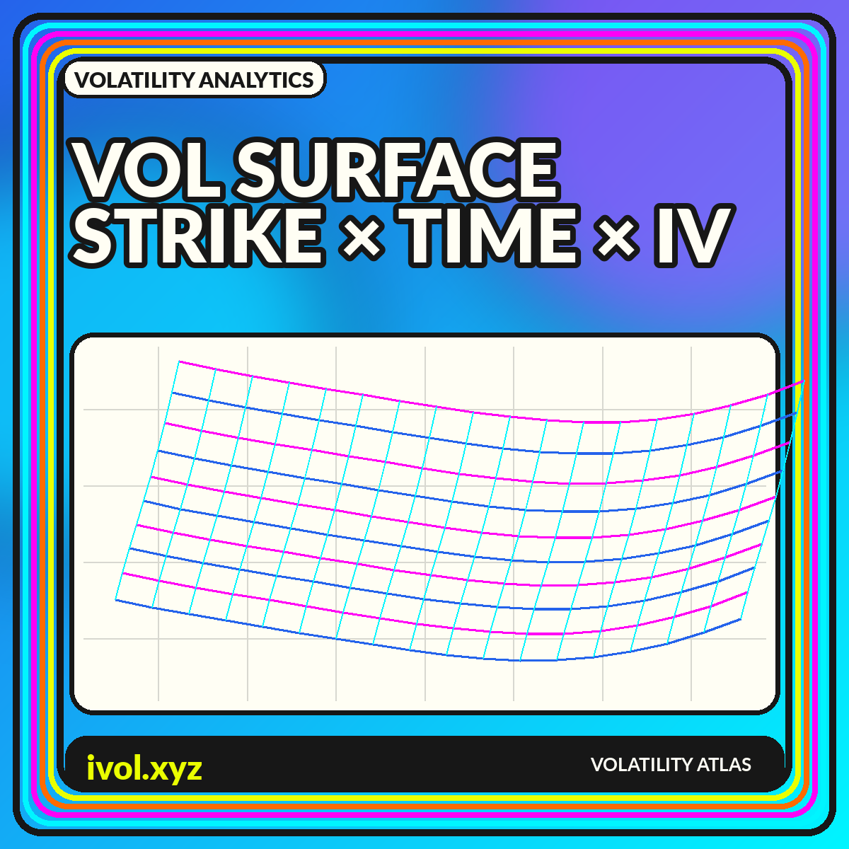
An implied-volatility quote belongs to an option with a strike and an expiration. Collect those quotes across the option chain and they form a surface: strike or moneyness on one axis, time to expiration on another, and implied volatility as height or color. The surface combines two familiar views. A slice across strikes shows skew or smile; a slice across expirations shows term structure. Looking at both dimensions helps reveal where the option market concentrates uncertainty and asymmetry.
The smooth surface shown on a screen is not the raw market. Listed options are discrete, quotes can be wide or stale, and interpolation fills the spaces between observations. Choices about forward price, dividends, rates, delta conventions, filters, and smoothing can change the shape. A trustworthy visualization therefore separates observed points from modeled regions and makes the construction visible. This guide focuses on reading the geometry without mistaking an elegant rendering for direct market truth.
The three dimensions of an implied-volatility surface
The horizontal strike dimension is often transformed into moneyness, log-moneyness, or option delta. Raw strike is intuitive for one snapshot but becomes difficult to compare after the underlying moves. Moneyness relates strike to spot or forward price, while delta maps options into probability-like exposure buckets under a model. The maturity dimension can be calendar dates, days to expiration, or year fractions. The vertical dimension is the implied volatility produced by a selected pricing and inversion method.
A surface plot should state all three conventions. “IV surface” alone is incomplete because a 25-delta put point and a strike at 90% of spot are not the same coordinate. For assets with dividends, funding costs, or carry, forward moneyness is often more coherent than spot moneyness. If the visualization mixes calls and puts, explain how put-call parity or an out-of-the-money selection rule was used to create a single curve at each maturity.
Skew, smile, and the shape across strikes
A volatility smile has higher implied volatility in both wings than near the center. A skew has a more directional slope, such as the familiar pattern in equity indexes where lower strikes often carry higher IV than higher strikes. The shape reflects priced asymmetry, tail risk, hedging demand, jumps, and model limitations. It should not be translated directly into a literal probability statement without specifying the assumptions used to recover a distribution.
Indexes designed around tail pricing can provide a complementary benchmark. The Cboe SKEW Index dashboard presents Cboe's SKEW Index, which is derived from S&P 500 option prices and is intended to describe perceived tail risk beyond what a symmetric volatility summary captures. A surface view can show where that asymmetry sits by maturity, while a single index compresses the information. Neither eliminates the need to inspect liquidity and the actual strike range behind the signal.
Term structure and event humps
A term-structure slice holds moneyness roughly constant and compares IV across expiration. Curves may slope upward, downward, or contain local humps. Scheduled events often lift the expiration that contains them because a finite amount of event variance is concentrated in that contract's life. After the event passes, the hump can collapse even if longer-term uncertainty remains. Broad stress can invert the front of the surface as near-term protection reprices sharply.
Calendar time and variance time should not be confused. Implied variance is approximately additive across non-overlapping periods under simplifying assumptions, while volatility is a square-root quantity. Comparing raw IV differences between two maturities can therefore obscure the event contribution. Variance-based charts or forward-volatility calculations can isolate the interval between expirations, but they amplify noise and depend on clean, comparable inputs. Label them as derived measures rather than direct quotes.
Observed quotes versus an interpolated surface
Option chains provide a lattice, not a continuous sheet. A surface engine filters quotes, solves for IV, and interpolates between the surviving points. Some systems fit each expiration separately and then smooth through time; others use a joint parametric model. The choice affects local curvature and extrapolation in illiquid wings. A glossy 3D mesh can hide sparse data, especially when only a few strikes have reliable two-sided markets.
Overlay observed nodes on the rendered surface and vary marker size by liquidity or spread. Use transparency or hatching for extrapolated regions. A residual chart—observed IV minus fitted IV—can reveal where smoothing misses the market. If the surface is used for risk, preserve bid and ask bounds rather than relying only on midpoints. A model value outside the executable market may look smooth but cannot be treated as a tradeable quote.
Data cleaning and no-arbitrage considerations
Stale quotes, zero bids, crossed markets, tiny premiums, and inconsistent timestamps can create implausible spikes. Filtering by spread, minimum price, volume, open interest, or quote age can improve stability, but aggressive filters may delete genuine tail information. The methodology should explain how it handles deep in- or out-of-the-money options and whether it uses calls, puts, or whichever side is out of the money.
A fitted surface can also violate basic arbitrage relationships if smoothing is performed independently at each point. Calendar spreads and butterfly relationships place constraints on option prices, not directly on a visually smooth IV sheet. Production models often incorporate constraints or diagnostic checks. Even for educational charts, warn when the surface is descriptive rather than arbitrage-free. Smoothness is an aesthetic property; economic consistency is a separate test.
2D heatmaps, slices, and 3D surfaces
Three-dimensional surfaces are visually compelling and useful for showing the concept, but perspective can obscure exact values and make steep areas appear larger depending on the camera angle. A two-dimensional heatmap places moneyness and maturity on a plane and uses color for IV. It is easier to scan and compare across dates, provided the color scale stays fixed. Contour lines can add readable thresholds without requiring a 3D view.
Slices remain essential. Show the current skew for selected maturities and the term structure for selected deltas. These plots expose local shape and exact labels better than a surface. A strong dashboard uses all three modes: heatmap for overview, slices for diagnosis, and optional 3D for exploration. Keep the same coordinate conventions and make crosshairs synchronize so a selected point can be traced across each view.
Comparing surfaces through time
Comparing two surfaces by eye is difficult because level shifts can dominate subtler shape changes. A difference surface subtracts the earlier IV from the later IV at matched coordinates. This highlights where the market repriced most, but only if both surfaces use the same maturity grid, moneyness convention, interpolation method, and observation time. Rolling expirations and changing spot prices make naive strike-by-strike subtraction unreliable.
For event analysis, compare constant days to expiration and delta buckets, or preserve actual listed expirations when the event date is the focus. Use a fixed color scale centered at zero for difference heatmaps. Small multiples can show the full before-and-after surfaces alongside the difference. Avoid animated rotations as the only comparison tool; motion is memorable but makes quantitative judgment harder and can hide changes on the far side of the mesh.
A practical surface-analysis workflow
Begin with a timestamped option chain and a documented forward estimate. Filter quotes with explicit rules, calculate IV consistently, and plot the surviving observations before fitting anything. Inspect each expiration's skew, then the at-the-money term structure. Fit or interpolate only after the raw data look credible. Save diagnostics such as spreads, point counts, and residuals with the surface snapshot.
When interpreting the result, separate level, slope, and curvature. Level describes the broad volatility regime. Strike slope captures asymmetry. Curvature describes wing richness, and term shape locates uncertainty in time. Compare those components with their own histories rather than using one surface screenshot as a trading conclusion. The surface is a compact map of option pricing, but the map remains conditional on the model and data pipeline that produced it.
Conclusion
A volatility surface organizes implied volatility across strike and expiration, revealing skew, smile, term structure, and event concentration in one framework. Its shape can be highly informative, but the continuous sheet is a model-assisted visualization built from discrete, imperfect quotes.
Show the observed nodes, state coordinate conventions, flag extrapolation, and include slice and residual views. Compare surfaces only on matched grids and consistent timestamps. With those safeguards, the surface becomes more than a dramatic 3D object: it becomes an auditable map of where and when the option market prices uncertainty.